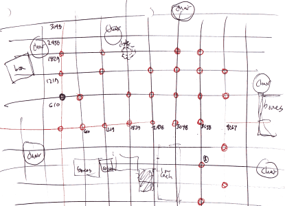
Figure 1. A hand-drawn map of the environment. Circles at intersections of the two-foot tiles show the locations where soundings were taken. [2514x1818 gif (262 KB)]
|
Gentle reader: This HTML document represents the submitted version
of the paper. The version printed in the proceedings includes our
results with more experiments, including using the algorithm to
determine orientation. See above for that paper
and related material.
The figures on this page correspond to those in the newer version of the paper, however, and are clearer for being in color. Figure 7 on this page also includes an animated GIF version showing more frames of the sequence. |
This paper describes an algorithm by which a robot can construct a map on the fly, and localize itself to its self-constructed map. This work was performed as my term project in Artificial Intelligence class, CS 104.
A robot should be able to navigate around a space with some persistent memory of the features of that space. In my system, the robot begins by taking a sonar sounding, which produces a polar distance map of the robot's immediate neighborhood. The robot is assumed to be at the origin (0,0), and these initial soundings are taken to be the robot's initial map.
Then the robot proceeds to move in some direction (goal planning is outside the scope of this project), stops, and takes another sounding. This sounding is fit to the existing map, on the assumption that the features in the robot's neighborhood have not changed much. The best fit returns a most likely location of the robot relative to the origin; the soundings are then shifted by the robot's now-known position, and contributed to the map. This cycle repeats indefinitely as the robot explores; at each stop, the soundings pointing ``behind'' the robot's path help it localize itself, and the soundings pointing ahead contribute new information to the map.
In this paper, I assume the robot has reliable orientation information, such as from a compass. It may have a few degrees of error, but that error does not accumulate as would error from a relative sensing system, such as odometry.
The algorithm presented here is based on Brown and Donald's idea of a ``feasible pose'' [BD96].
The data used in this experiment were collected from the RWI B14 robot named bonnie that resides in the Dartmouth Robotics Lab. The environment consists of the assorted desks, chairs, robots, and cardboard boxes that were strewn about the lab on Thursday, May 27, 1999. The robot has sixteen sonar transducers evenly spaced 22.5° apart. By rotating the robot's body to each of {0°, 6°, 11°, 17°} and taking soundings from every sensor, I simulated a ring of sixty-four sensors at 5.6° spacing.
A sonar sensor measures the time-of-flight of a burst of sound. Sonar can see a ``cone'' of about 22° arc, so it blurs the boundaries of the objects it sees. The return value is a single number representing the first echo above some threshold amplitude, so the blur is a box convolution. If sonar hits a surface at a wide angle from the surface normal, the signal may not return, or it may bounce off a second surface and produce a ``ghost'' image.
The algorithm is meant to be an online algorithm, but I built and tested it in an offline fashion. I manually placed the robot at twenty-eight different locations in the lab, and took soundings of the sonar surface around the robot at each location. In each case, I positioned the robot over the intersection of the steel floor tiles, so I knew its position to within about a centimeter, and its orientation to within a few degrees (see Figure 1).
Figure 1.
A hand-drawn map of the environment. Circles at
intersections of the two-foot tiles show the locations where
soundings were taken.
[2514x1818 gif (262 KB)]
I calibrated the sonar by placing a box at known distances from 1 m to 4 m from the robot, and reading the sonar value. The returned values and the known values had a very close to linear relationship, which is not surprising: sound travels at a constant speed, and time is one quantity we can ``sense'' with high precision (see Figure 2). All of the sonar soundings were mapped through the measured linear function to produce a distance value in millimeters. I also produced a histogram of the entire collection of 7,616 sonar readings, shown in Figure 3. Low values (less than 200) are reflections from the cables hanging off the robot; high values are always 16384, a sentinel meaning ``no echo received.'' These thresholds were used to remove useless values from the input data.
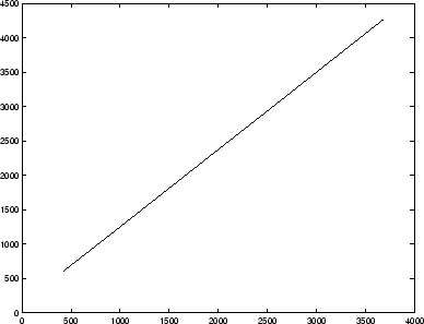
Figure 2.
The relationship between returned sonar values and
actual measured distance is very close to linear.
[eps (7 KB)]
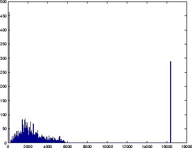
Figure 3.
A histogram of 7168 sonar readings taken around the room,
showing low and high garbage values.
[eps (135 KB)]
The first experiment, described in Section 3, compares the robot's determination of its position with the position I recorded.
In the second experiment, described in Section 4, only soundings from successive positions of the robot are considered in the algorithm. The computed position of the robot is used to locate the robot in the map and contribute the new soundings to the map. The positions are sorted by distance from the origin, simulating the robot growing its map slowly by ``pushing the envelope'' of the well-mapped area. Therefore, this second experiment approximates online behavior in the sense that the algorithm has access to no data that it wouldn't have had otherwise. Actually performing the algorithm online did not make sense for two reasons: First, I did not want to spend time figuring out how to ship data between the robots and the workstation running MatLab. Second, it was much easier to tweak the algorithm and re-run it on stored data than to wait many minutes for the robot to take new soundings of the same environment.
The first experiment was designed to determine how well the robot could find itself in an existing map given only a set of sonar readings and a known orientation. The experiment consisted of 28 trials. In each one, the sonar readings from one of the 28 positions was removed into a test set. The remaining readings, together with the known location of the robot when each was taken, became the ``known map'' (see Figure 4). Some fraction (frequently 3/16) of all sonar readings was discarded to make the algorithm run more quickly.
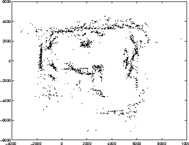
Figure 4.
The known map: all 6414 valid sonar readings. Each
vector points back at the position of the robot when that
reading was taken; the vector's distance from the robot's position
is equal to the distance value sensed by sonar.
[eps (380 KB)]
The test set of sonar readings consists of angles and distances from the robot's center, but the robot's location relative to the map is unknown. So, I compare each test sonar value with every map vector. The map vectors represent the position and the very approximate normal of some observed surface in the environment. Therefore, those pairs of <test vector, map vector > that did not agree to within some threshold (I chose 30°) were discarded. The idea is that a map vector represents the ``front'' of some object in the room; it is unlikely that a test vector could ``see'' that surface from behind or from a shallow angle.
The remaining pairs ``vote'' for the ``most feasible'' (likely) pose of the robot. The position of the map vector is added to the negative of the test vector to locate where the robot would have to have been for the test vector to represent a reflection off of the same surface responsible for the map vector. Each vote contributes a small value to a raster image. The location with the most votes is taken to be the most likely location of the robot. See Figure 5.
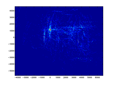
Figure 5.
A collection of votes. Brighter spots received more votes.
[eps (131 KB)]
This transformation is analogous to the Hough transform, which ``finds'' lines (or other geometry) by letting each point in an image vote for the feasible lines, those that can pass through that point. Essentially, my algorithm is a Hough transform for the star shape made by the points of the test vector.
The surface of votes is very spiky, due to the sporadic nature of sonar samples of the environment. In fact, the map vectors can only be considered a guess at the location of the reflecting surface, because of the signal blur mentioned earlier. Therefore, I convolve the vote raster with a two-dimensional Gaussian surface to smooth it out. Figure 6 shows the smoothed vote surface superimposed with the known map (short vectors) and the star-shaped test vectors, translated to the location of the maximum value on the vote surface.
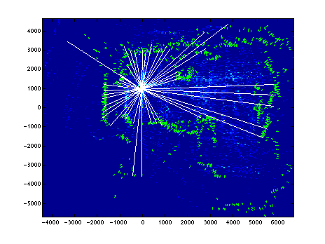
Figure 6.
A successful localization.
[eps (201 KB)]
To quantify the reliability of this algorithm, I ran it for all 28 test vectors, and repeated each run with 1/16, 2/16, and 3/16 of the map data. The results are displayed in Table 1.
A ``wild error'' is an error more than half a meter away from the known location where the sample was originally taken. Generally, these occurred when the sample was taken in a sparsely-populated corner of the map (the lower right corridor), and an approximate match in a heavily-populated section was able to outvote the correct position. These gross errors could be easily detected by using auxiliary sensing such as odometry. I propose a solution to this problem in Section 6.2.
The remaining errors (``tame errors'') have a mean of 50 to 90 millimeters, depending on how much sonar data was used in the map. Increasing the resolution of the raster gave a small improvement in the accuracy of the algorithm. Doubling the resolution quadruples the size of the raster, which slows the convolution and maximum-finding phases of the algorithm; however, with the parameters presented here, the vote-collecting phase dominates the total run time.
The previous experiment introduced the voting algorithm for localization, and demonstrated that it is practical. However, it assumed the existence of a rich map already available. An on-line algorithm would need to be able to construct a map from successive localization--map marking cycles. To simulate this, I ran the following experiment. I started by taking the sonar readings from (0,0) as an initial map. The remaining locations were sorted by increasing distance from the origin. For each location in turn, the corresponding sonar data were taken as the test vectors, used to localize the robot, and the output of the algorithm used to translate the test vectors and add them to the map. This simulated the robot moving to locations on the outskirts of its explored territory, using inward-looking vectors to localize itself, and contributing the outward vectors to its map.
Figure 7 shows snapshots of the map at various stages of growth.
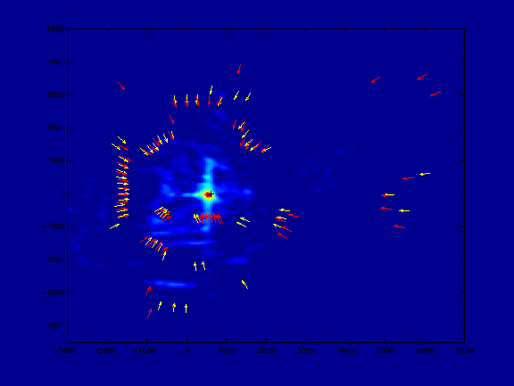
Figure 7.
An online mapping sequence. Long vectors are test vectors
that have been localized against the short (map) vectors; in the
next round of the algorithm, the localized test vectors join the
rest of the map.
[animated gif (16 frames, 231 KB)]
From the experiments, I learned that a voting algorithm can reliably find a match in an existing map for a sensed sonar contour. The shortcomings of the algorithm are its speed and the ``wild'' errors. I discuss proposed solutions to both problems in Section 6.
I was surprised by the effectiveness of this simple algorithm. When I have the opportunity, I would like to extend it further by extending it to handle orientation localization, modifying it to exhibit real-time performance, and then trying it online on a self-navigating robot.
The algorithm assumes that the orientation of the robot is known. This is reasonable because electronic compasses are inexpensive and readily available. However, compasses can often be confused by the metal structure of buildings. One straightforward way to detect orientation information is to run the same algorithm repeatedly with the test vectors rotated to a selection of angles, and take the maximum over all of the voting surfaces. This might be performed in two steps, once at low resolution, and once at high resolution once the approximate angle is known. Or, if the robot has an estimate of its orientation (using odometry), it may only need to be run at high resolution but over a limited choice of angles.
6.2 Limiting the problem size
The algorithm slows linearly in the number of vectors in the map.
To combat this, I propose three solutions: restricting the map to
the neighborhood of the robot, thinning the map, and aging old map data away.
Neighborhood reduction. If the robot has not traveled far from a previously localized position, there is no need to consider map vectors that cannot be reached by any of the test vectors. This neighborhood can be reduced even further if the robot's odometry provides even gross information about the robot's new position relative to its previous localization. The latter step will also reduce the opportunities for wild errors.
Density reduction. The thinning operation described earlier the paper can be used to reduce the amount of data being inspected. One might set a limit on the number of map vectors to be inspected (the number needed to reasonably represent the surfaces in a neighborhood as described previously), and then select that many vectors at random from the neighborhood to participate in the voting.
Temporal reduction. The previous suggestion involves discarding map data at random; however, more recently-acquired data is more likely to be valid than older data. Therefore, recent map data should have a higher likelihood of participating in the voting process. This has the advantage that stale information (such as the image of a chair that has since been moved) will gradually fade from the map, while current information will be reinforced by repeated observations.
I would like to try the online experiment actually online. In addition to the orientation localization and the performance improvements described above, this extension would involve creating a basic motion planner for the robot. Given the collection of sonar samples, it would make sense to plan based on a probabilistic rasterized occupancy grid. To encourage exploration, the robot would be drawn toward unpopulated portions of the map.
[BD96] Russell G. Brown and Bruce R. Donald. Mobile robot self-localization without explicit landmarks. Algorithmica, November 1996. To appear.